Lagrange points
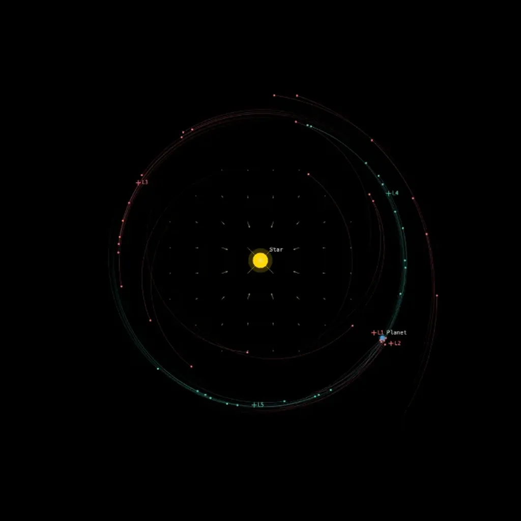
This simulation needs WebAssembly, and it could not start in this browser.
The image is a frame from a real run. Check that JavaScript is on, or try another browser.
Two bodies on circular orbits around each other have five points where a third, much lighter body can stay at rest relative to them. Leonhard Euler found the three on the line through the two masses around 1767, and Joseph-Louis Lagrange the two that form equilateral triangles with them in 1772. Spacecraft and asteroids use them: the James Webb Space Telescope circles the Sun-Earth point , 1.5 million km beyond the Earth, and thousands of Trojan asteroids share Jupiter’s orbit around and , 60° ahead of and behind the planet.
What you see
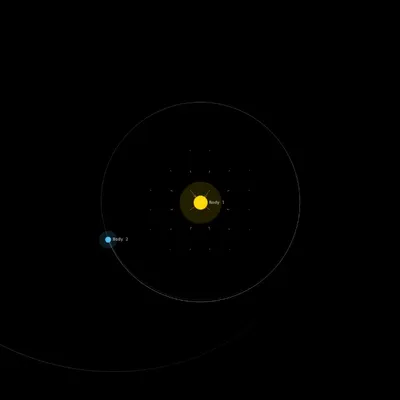
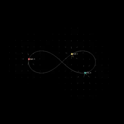
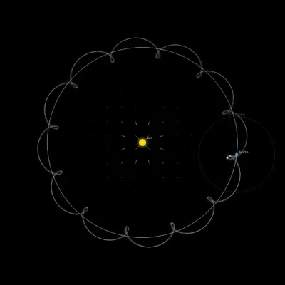
A star (yellow) of mass and a planet (blue) of mass move on circular orbits around their center of mass, one unit apart. Ten massless test particles start near each Lagrange point, scattered by up to 0.02 in position and 0.002 in velocity from exact co-rotation. Particles from the unstable points , and are red, those from and teal. Small crosses mark the five points and turn with the planet.
By default the view is the inertial frame, so the whole pattern rotates. Set corot. ω to 1 to rotate the canvas with the orbit: the star and planet then stand still, and you can watch each particle drift away from its Lagrange point or loop around it.
Governing equation
The simulation integrates Newtonian gravity in the inertial frame, with , total mass 1 and separation 1, so the orbital angular velocity is 1 and the period . In the frame that rotates with the orbit, a test particle feels the effective potential
plus the Coriolis force , where and are the distances to the star and the planet. The Lagrange points are the five stationary points of . The simulation places them at
with the Hill radius ; the first three are the leading terms for small .
, and are saddle points and always unstable. and are maxima of , yet the Coriolis force turns a particle sliding off them into a loop around the point. This works only below the Routh limit:
Presets
The four presets start the same way and differ only in . Over about fifty orbits they behave as follows.
Sun-Jupiter (Trojans): . The red particles next to the planet, at and , are scattered within a few orbits; those at , where the instability is weak, drift away slowly. Most teal particles stay near and on wide, tadpole-shaped loops.
Sun-Earth (JWST at L2): . Here and lie only 0.01 from the planet, closer than the spread of the starting positions. The planet is too light to hold even the teal particles against offsets this large, and most of them drift away along the orbit. JWST itself stays near only with a small engine burn every few weeks.
Earth-Moon: , the Moon’s share of the Earth-Moon mass. Of all four presets, the teal particles stay closest to their points here.
Near Routh limit (μ=0.037): just below the threshold. Linear theory still predicts stability, but the margin is thin: about half the teal particles escape, and the rest circle their points in wide loops.
Parameters
mass ratio μ: the planet’s share of the total mass, 0.0001 to 0.038 (default 0.001).
corot. ω: rotates the view at this angular velocity, from -3 to 3 (default 0); a value of 1 follows the orbit. It changes only the drawing.
trail length: 0 to 1000 steps (default 300); trails switches them off.
integrator and softening: leapfrog and by default. The time step is fixed at 0.005.
The remaining controls change only the drawing: labels, the center-of-mass marker, a view locked to the center of mass, velocity arrows and the field overlays.