Lissajous figures
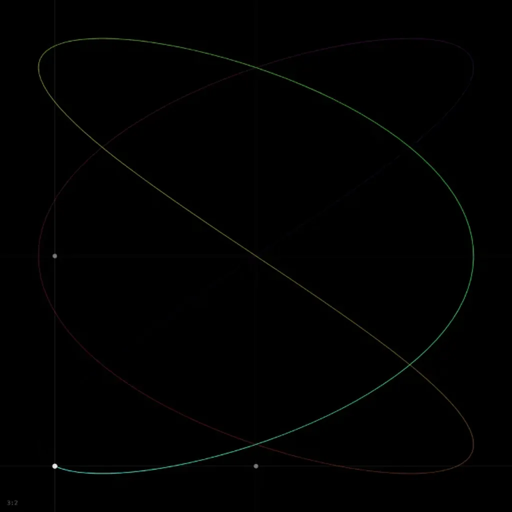
This simulation needs WebAssembly, and it could not start in this browser.
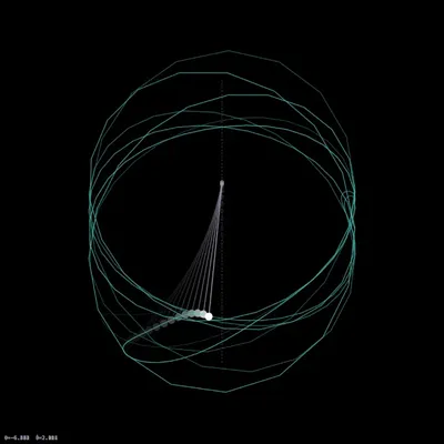
The image is a frame from a real run. Check that JavaScript is on, or try another browser.
Combine two perpendicular oscillations and the moving point traces a Lissajous figure. Nathaniel Bowditch studied these curves with a compound pendulum in 1815. In 1857 Jules Antoine Lissajous made them visible by reflecting a beam of light off mirrors fixed to two tuning forks vibrating at right angles, and used the figures to compare the forks’ frequencies. When the two frequencies are in a ratio of small integers, the curve closes and its shape tells you the ratio at a glance.
What you see
The point with a trail of its last 2000 steps, colored in a rainbow that slowly cycles, older parts dimmer and the current position as a white dot. With axis projections on, faint lines run through the dot, and two small markers on the center lines show and on their own. The ratio is shown at the bottom left.
The presets set only the ratio and keep the current phase and decay. At the default phase δ = π/2:
1:1 gives a circle.
2:1 collapses into a parabola, , traced back and forth.
3:2 is a closed curve with crossings that touches the left and right edges three times each and the top and bottom twice each.
4:3, 5:4, 5:3, 3:1, 4:1, 5:2: denser figures following the same rule. Those with an even and an odd (4:3 and 4:1) collapse into an open arc traced back and forth, like 2:1; most other phases open them into closed curves.
Governing equation
The simulation integrates two independent damped oscillators,
started so that without damping
The slider values for and are integers that multiply a base frequency of 1.2 rad/s, so every figure closes after s when the two integers have no common factor. For coprime integers the closed curve touches each side edge times and the top and bottom edges times. With damping the amplitude falls as and the curve winds into the center. The default integrator is fourth-order Runge-Kutta.
Parameters
ωₓ, ωᵧ: integers from 1 to 9, defaults 3 and 2.
phase δ (×π): the phase of the horizontal oscillation in units of π, 0 to 2, default 0.5.
decay γ (s⁻¹): the amplitude decay rate, 0 to 0.5, default 0.
timestep dt: 0.005 to 0.1, default 0.02. The simulation takes one step per frame, so dt sets how fast the figure is drawn and how much of it the trail covers.